BTER Guide: How to create a BTER graph for benchmarking

By the BTER Team (Sandia National Laboratories, Livermore, CA):

April 2013

Distributed with href="index.html">FEASTPACK</a.

Abstract: The attached document shows how to create BTER models for benchmarking, following the reference given at the end of the document.

Sandia National Laboratories is a multi-program laboratory managed and operated by Sandia Corporation, a wholly owned subsidiary of Lockheed Martin Corporation, for the U.S. Department of Energy's National Nuclear Security Administration under contract DE-AC04-94AL85000.

Contents

Step 1: Decide characteristics of the graph

BTER requires a degree distribution and clustering coefficient by degree profile as input. We'll derive these based on some overall graph metrics:

nnodes = 1e5; % Number of nodes
maxdeg_bound = 1e4; % Absolute bound on maximum degree
avgdeg_target = 32; % Target average degree
maxccd_target = 0.95; % Target maximum clustering coefficient (for degree 2)
gcc_target = 0.15; % Target global clustering coefficient

Step 2: Create a desired degree distribution

We need to proscribe a specific degree distribution. We recommend the discrete generalized log normal, but we also provide the option to use the discrete power law (discussed below). The generalized log normal distribution says that the probability of degree $d$ is

$P(d \,|\, \alpha, \beta) \propto \exp\left[-\left(\frac{\log d}{\alpha}\right)^\beta\right],$

where $\alpha$ and $\beta$ are parameters of the distribution. Similarily, the power law distribution says that the probability of degree $d$ is

$P(d \,|\, \gamma) \propto d^{-\gamma},$

where $\gamma$ is the parameter of the distribution.

We require the distribution to be discrete and let $d^*$ denote the absolute bound on maximum degree (denoted as maxdeg_bound in the code). For any distribution, we set $P(d) = 0$ for all $d > d^*$ and then normalize so that $\sum_{d=1}^{d_*} P(d) = 1$.

Our goal is to find parameters for the selected distribution such that the following hold:

We provide the function degdist_param_search which uses optimization to search for parameters that meet the above two objectives. Specifically, it tries to minimize the function $f = f_1 + f_2$ where

$f_1 = \left\{ \begin{array}{ll} \left[\exp\left(1 + P(d^*) - \tau \right) \right]^2 - 1, & \mbox{if } P(d^*) > \tau \\ 0, & \mbox{otherwise} \end{array} \right. \quad\mbox{and}\quad f_2 = \left[ \bar d - \left(\sum_{d=1}^{d^*} d \cdot P(d) \right) \right]^2.$

Here, $\bar d$ represents the desired average degree (denoted as avgdeg_target in the code). The value of $\tau$ should be less than $1/n$ and defaults to 1e-10. It can be modified via the 'maxdeg_prbnd' option of degdist_param_search.

% Run the optimization procedure
tau = 1e-3 / nnodes; % tau << 1/nnodes
[alpha, beta] = degdist_param_search(avgdeg_target, maxdeg_bound, 'maxdeg_prbnd', tau);
fprintf('Selected alpha=%f and beta=%f\n', alpha, beta);

alpha=2.000, beta=2.000, maxdeg=10000, p(maxdeg)=6.568451e-11, avgdeg=20.6, y=129.32
alpha=2.100, beta=2.000, maxdeg=10000, p(maxdeg)=4.044975e-10, avgdeg=28.0, y=16.25
alpha=2.000, beta=2.100, maxdeg=10000, p(maxdeg)=2.113216e-12, avgdeg=15.7, y=265.65
alpha=2.100, beta=1.900, maxdeg=10000, p(maxdeg)=5.206135e-09, avgdeg=42.5, y=110.20
alpha=2.200, beta=1.900, maxdeg=10000, p(maxdeg)=1.793480e-08, avgdeg=61.2, y=856.82
alpha=2.050, beta=1.975, maxdeg=10000, p(maxdeg)=3.490557e-10, avgdeg=26.2, y=34.06
alpha=2.050, beta=2.075, maxdeg=10000, p(maxdeg)=1.601137e-11, avgdeg=19.1, y=165.74
alpha=2.087, beta=1.944, maxdeg=10000, p(maxdeg)=1.486064e-09, avgdeg=33.4, y=1.96
alpha=2.138, beta=1.969, maxdeg=10000, p(maxdeg)=1.661232e-09, avgdeg=35.6, y=12.74
alpha=2.125, beta=1.913, maxdeg=10000, p(maxdeg)=5.419218e-09, avgdeg=43.8, y=138.18
alpha=2.106, beta=1.978, maxdeg=10000, p(maxdeg)=8.096126e-10, avgdeg=30.9, y=1.12
alpha=2.056, beta=1.953, maxdeg=10000, p(maxdeg)=7.118139e-10, avgdeg=29.0, y=9.06
alpha=2.077, beta=1.957, maxdeg=10000, p(maxdeg)=8.867045e-10, avgdeg=30.5, y=2.22
alpha=2.117, beta=1.965, maxdeg=10000, p(maxdeg)=1.354375e-09, avgdeg=33.8, y=3.23
alpha=2.087, beta=1.959, maxdeg=10000, p(maxdeg)=9.876731e-10, avgdeg=31.3, y=0.49
alpha=2.105, beta=1.993, maxdeg=10000, p(maxdeg)=5.312901e-10, avgdeg=29.1, y=8.15
alpha=2.092, beta=1.956, maxdeg=10000, p(maxdeg)=1.154441e-09, avgdeg=32.2, y=0.05
alpha=2.072, beta=1.937, maxdeg=10000, p(maxdeg)=1.408339e-09, avgdeg=32.7, y=0.43
alpha=2.078, beta=1.934, maxdeg=10000, p(maxdeg)=1.640504e-09, avgdeg=33.6, y=2.72
alpha=2.084, beta=1.953, maxdeg=10000, p(maxdeg)=1.122558e-09, avgdeg=31.9, y=0.02
alpha=2.104, beta=1.972, maxdeg=10000, p(maxdeg)=9.204847e-10, avgdeg=31.5, y=0.28
alpha=2.096, beta=1.963, maxdeg=10000, p(maxdeg)=1.023617e-09, avgdeg=31.7, y=0.07
alpha=2.080, beta=1.946, maxdeg=10000, p(maxdeg)=1.266152e-09, avgdeg=32.3, y=0.11
alpha=2.092, beta=1.959, maxdeg=10000, p(maxdeg)=1.079473e-09, avgdeg=31.9, y=0.01
alpha=2.085, beta=1.955, maxdeg=10000, p(maxdeg)=1.049334e-09, avgdeg=31.5, y=0.22
alpha=2.090, beta=1.956, maxdeg=10000, p(maxdeg)=1.127320e-09, avgdeg=32.0, y=0.00
alpha=2.098, beta=1.962, maxdeg=10000, p(maxdeg)=1.084245e-09, avgdeg=32.1, y=0.01
alpha=2.096, beta=1.959, maxdeg=10000, p(maxdeg)=1.132159e-09, avgdeg=32.2, y=0.05
alpha=2.093, beta=1.959, maxdeg=10000, p(maxdeg)=1.092435e-09, avgdeg=32.0, y=0.00
alpha=2.085, beta=1.953, maxdeg=10000, p(maxdeg)=1.136011e-09, avgdeg=31.9, y=0.00
alpha=2.089, beta=1.955, maxdeg=10000, p(maxdeg)=1.122774e-09, avgdeg=32.0, y=0.00
alpha=2.091, beta=1.958, maxdeg=10000, p(maxdeg)=1.087994e-09, avgdeg=31.9, y=0.01
alpha=2.090, beta=1.957, maxdeg=10000, p(maxdeg)=1.117361e-09, avgdeg=32.0, y=0.00
alpha=2.086, beta=1.953, maxdeg=10000, p(maxdeg)=1.148455e-09, avgdeg=32.0, y=0.00
alpha=2.088, beta=1.954, maxdeg=10000, p(maxdeg)=1.142888e-09, avgdeg=32.0, y=0.00
alpha=2.088, beta=1.955, maxdeg=10000, p(maxdeg)=1.127770e-09, avgdeg=32.0, y=0.00
alpha=2.088, beta=1.954, maxdeg=10000, p(maxdeg)=1.137827e-09, avgdeg=32.0, y=0.00
alpha=2.088, beta=1.955, maxdeg=10000, p(maxdeg)=1.130277e-09, avgdeg=32.0, y=0.00
alpha=2.093, beta=1.959, maxdeg=10000, p(maxdeg)=1.099729e-09, avgdeg=32.0, y=0.00
alpha=2.091, beta=1.957, maxdeg=10000, p(maxdeg)=1.112414e-09, avgdeg=32.0, y=0.00
alpha=2.091, beta=1.957, maxdeg=10000, p(maxdeg)=1.116122e-09, avgdeg=32.0, y=0.00
alpha=2.091, beta=1.957, maxdeg=10000, p(maxdeg)=1.113649e-09, avgdeg=32.0, y=0.00
alpha=2.091, beta=1.957, maxdeg=10000, p(maxdeg)=1.115503e-09, avgdeg=32.0, y=0.00
alpha=2.086, beta=1.953, maxdeg=10000, p(maxdeg)=1.146544e-09, avgdeg=32.0, y=0.00
alpha=2.091, beta=1.957, maxdeg=10000, p(maxdeg)=1.111228e-09, avgdeg=32.0, y=0.00
alpha=2.088, beta=1.954, maxdeg=10000, p(maxdeg)=1.134634e-09, avgdeg=32.0, y=0.00
alpha=2.089, beta=1.955, maxdeg=10000, p(maxdeg)=1.128731e-09, avgdeg=32.0, y=0.00
alpha=2.091, beta=1.957, maxdeg=10000, p(maxdeg)=1.113981e-09, avgdeg=32.0, y=0.00
alpha=2.089, beta=1.955, maxdeg=10000, p(maxdeg)=1.126177e-09, avgdeg=32.0, y=0.00
alpha=2.087, beta=1.954, maxdeg=10000, p(maxdeg)=1.139548e-09, avgdeg=32.0, y=0.00
alpha=2.085, beta=1.952, maxdeg=10000, p(maxdeg)=1.151790e-09, avgdeg=32.0, y=0.00
alpha=2.087, beta=1.954, maxdeg=10000, p(maxdeg)=1.136967e-09, avgdeg=32.0, y=0.00
alpha=2.088, beta=1.955, maxdeg=10000, p(maxdeg)=1.130784e-09, avgdeg=32.0, y=0.00
alpha=2.088, beta=1.954, maxdeg=10000, p(maxdeg)=1.134902e-09, avgdeg=32.0, y=0.00
alpha=2.088, beta=1.955, maxdeg=10000, p(maxdeg)=1.131812e-09, avgdeg=32.0, y=0.00
alpha=2.086, beta=1.953, maxdeg=10000, p(maxdeg)=1.145258e-09, avgdeg=32.0, y=0.00
alpha=2.088, beta=1.955, maxdeg=10000, p(maxdeg)=1.130914e-09, avgdeg=32.0, y=0.00
alpha=2.087, beta=1.954, maxdeg=10000, p(maxdeg)=1.140454e-09, avgdeg=32.0, y=0.00
alpha=2.088, beta=1.954, maxdeg=10000, p(maxdeg)=1.132710e-09, avgdeg=32.0, y=0.00
alpha=2.087, beta=1.954, maxdeg=10000, p(maxdeg)=1.137835e-09, avgdeg=32.0, y=0.00
alpha=2.088, beta=1.955, maxdeg=10000, p(maxdeg)=1.129215e-09, avgdeg=32.0, y=0.00
alpha=2.088, beta=1.955, maxdeg=10000, p(maxdeg)=1.132013e-09, avgdeg=32.0, y=0.00
alpha=2.089, beta=1.955, maxdeg=10000, p(maxdeg)=1.126025e-09, avgdeg=32.0, y=0.00
alpha=2.088, beta=1.954, maxdeg=10000, p(maxdeg)=1.134869e-09, avgdeg=32.0, y=0.00
alpha=2.088, beta=1.954, maxdeg=10000, p(maxdeg)=1.134667e-09, avgdeg=32.0, y=0.00
alpha=2.088, beta=1.954, maxdeg=10000, p(maxdeg)=1.132676e-09, avgdeg=32.0, y=0.00
alpha=2.087, beta=1.954, maxdeg=10000, p(maxdeg)=1.135736e-09, avgdeg=32.0, y=0.00
alpha=2.088, beta=1.954, maxdeg=10000, p(maxdeg)=1.132791e-09, avgdeg=32.0, y=0.00
alpha=2.088, beta=1.955, maxdeg=10000, p(maxdeg)=1.130602e-09, avgdeg=32.0, y=0.00
alpha=2.088, beta=1.955, maxdeg=10000, p(maxdeg)=1.131667e-09, avgdeg=32.0, y=0.00
alpha=2.088, beta=1.955, maxdeg=10000, p(maxdeg)=1.131783e-09, avgdeg=32.0, y=0.00
alpha=2.088, beta=1.955, maxdeg=10000, p(maxdeg)=1.132452e-09, avgdeg=32.0, y=0.00
alpha=2.088, beta=1.955, maxdeg=10000, p(maxdeg)=1.132006e-09, avgdeg=32.0, y=0.00
alpha=2.088, beta=1.955, maxdeg=10000, p(maxdeg)=1.132341e-09, avgdeg=32.0, y=0.00
alpha=2.088, beta=1.954, maxdeg=10000, p(maxdeg)=1.133465e-09, avgdeg=32.0, y=0.00
alpha=2.088, beta=1.954, maxdeg=10000, p(maxdeg)=1.133016e-09, avgdeg=32.0, y=0.00
Selected alpha=2.087916 and beta=1.954470

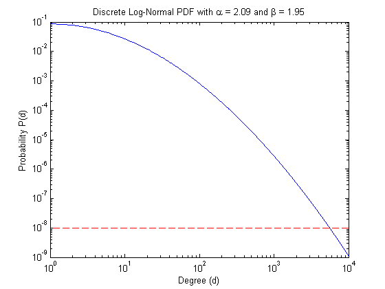
Now that we have target values, we can create the distribution and visualize it. The red dashed line shows the cutoff value of $\tau$.

% Create the discrete PDF
pdf = dglnpdf(maxdeg_bound,alpha,beta);

% Visualize the PDF
figure;
loglog(pdf);
hold on;
plot([1 maxdeg_bound], [tau tau], 'r--');
tstr = sprintf('Discrete Log-Normal PDF with \\alpha = %.2f and \\beta = %.2f', alpha, beta);
title(tstr);
xlabel('Degree (d)')
ylabel('Probability P(d)');

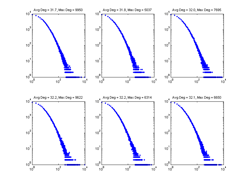
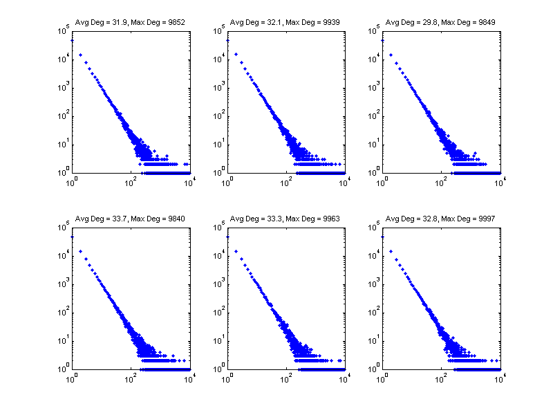
Now we show a few realizations of the sampled degree distribution, denoted by nd in the code. We'll use the last one as we move forward to Step 3.

figure;
pos = get(gcf, 'Position');
set(gcf, 'Position', [pos(1) pos(2) 800 600]);
for i = 1:6
    subplot(2,3,i);
    set(gca, 'FontSize', 8);
    nd = gendegdist(nnodes,pdf);
    loglog(nd,'b.');
    xlim([1 maxdeg_bound])
    avgdeg = sum(nd .* (1:length(nd))')/sum(nd);
    maxdeg = find(nd>0,1,'last');
    tstr = sprintf('Avg Deg = %.1f, Max Deg = %d', avgdeg, maxdeg);
    title(tstr);
end

Step 3: Create a desired clustering coefficient per degree profile

We have wide latitude in choosing the clustering coefficients. Let $\{n_d\}$ be the specified degree distribution (denoted as nd in the code). Then we use the following arbitrary formula to define the clustering coefficient profile:

$\bar c_d = c_{\rm max} \exp[-(d-1) \cdot \xi] \mbox{ for } d \geq 2,$

where $c_{\rm max}$ and $\xi$ are user-defined parameters. We've already specified $c_{\rm max}$ with the choice of maxccd_target. We let ccd_target denote $\bar c_d$ and xi denote $\xi$. We provide the function cc_param_search to determine $\xi$, based on the target GCC value.

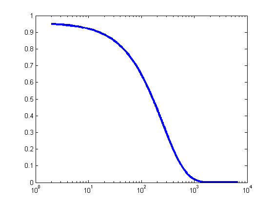
% Find the optimal xi
maxdeg = find(nd>0,1,'last');
xi = cc_param_search(nd, maxccd_target, gcc_target);
fprintf('Selected xi=%f\n', xi);

% Plot the target clustering coefficient per degree (CCD)
ccd_target = [0; maxccd_target * exp(-(0:maxdeg-2)'.* xi)];
figure;
semilogx(2:maxdeg, ccd_target(2:end),'LineWidth',3);
hold on;
ylim([0,1]);
xlim([1 maxdeg_bound]);

xi = 5.000000e-01, target gcc = 0.150000, current gcc = 0.000138
xi = 5.250000e-01, target gcc = 0.150000, current gcc = 0.000127
xi = 4.750000e-01, target gcc = 0.150000, current gcc = 0.000150
xi = 4.500000e-01, target gcc = 0.150000, current gcc = 0.000165
xi = 4.000000e-01, target gcc = 0.150000, current gcc = 0.000203
xi = 3.500000e-01, target gcc = 0.150000, current gcc = 0.000256
xi = 2.500000e-01, target gcc = 0.150000, current gcc = 0.000468
xi = 1.500000e-01, target gcc = 0.150000, current gcc = 0.001162
xi = -5.000000e-02, target gcc = 0.150000, current gcc = 94536884188130833000000000000000000000000000000000000000000000000000000000000000000000000000000000000000000000000000000000000000000000000000000.000000
xi = 2.500000e-01, target gcc = 0.150000, current gcc = 0.000468
xi = 5.000000e-02, target gcc = 0.150000, current gcc = 0.007180
xi = -5.000000e-02, target gcc = 0.150000, current gcc = 94536884188130833000000000000000000000000000000000000000000000000000000000000000000000000000000000000000000000000000000000000000000000000000000.000000
xi = -5.000000e-02, target gcc = 0.150000, current gcc = 94536884188130833000000000000000000000000000000000000000000000000000000000000000000000000000000000000000000000000000000000000000000000000000000.000000
xi = 1.000000e-01, target gcc = 0.150000, current gcc = 0.002340
xi = -4.440892e-16, target gcc = 0.150000, current gcc = 0.950000
xi = 7.500000e-02, target gcc = 0.150000, current gcc = 0.003775
xi = 2.500000e-02, target gcc = 0.150000, current gcc = 0.019552
xi = -4.440892e-16, target gcc = 0.150000, current gcc = 0.950000
xi = -4.440892e-16, target gcc = 0.150000, current gcc = 0.950000
xi = 3.750000e-02, target gcc = 0.150000, current gcc = 0.011052
xi = 1.250000e-02, target gcc = 0.150000, current gcc = 0.046725
xi = -4.440892e-16, target gcc = 0.150000, current gcc = 0.950000
xi = -4.440892e-16, target gcc = 0.150000, current gcc = 0.950000
xi = 1.875000e-02, target gcc = 0.150000, current gcc = 0.028521
xi = 6.250000e-03, target gcc = 0.150000, current gcc = 0.098027
xi = -4.440892e-16, target gcc = 0.150000, current gcc = 0.950000
xi = -4.440892e-16, target gcc = 0.150000, current gcc = 0.950000
xi = 9.375000e-03, target gcc = 0.150000, current gcc = 0.064546
xi = 3.125000e-03, target gcc = 0.150000, current gcc = 0.181043
xi = -4.440892e-16, target gcc = 0.150000, current gcc = 0.950000
xi = -4.440892e-16, target gcc = 0.150000, current gcc = 0.950000
xi = 4.687500e-03, target gcc = 0.150000, current gcc = 0.128429
xi = 6.250000e-03, target gcc = 0.150000, current gcc = 0.098027
xi = 3.906250e-03, target gcc = 0.150000, current gcc = 0.150684
xi = 3.125000e-03, target gcc = 0.150000, current gcc = 0.181043
xi = 4.296875e-03, target gcc = 0.150000, current gcc = 0.138761
xi = 3.515625e-03, target gcc = 0.150000, current gcc = 0.164596
xi = 4.101562e-03, target gcc = 0.150000, current gcc = 0.144501
xi = 3.710937e-03, target gcc = 0.150000, current gcc = 0.157361
xi = 4.003906e-03, target gcc = 0.150000, current gcc = 0.147534
xi = 3.808594e-03, target gcc = 0.150000, current gcc = 0.153957
xi = 3.955078e-03, target gcc = 0.150000, current gcc = 0.149094
xi = 3.857422e-03, target gcc = 0.150000, current gcc = 0.152305
xi = 3.930664e-03, target gcc = 0.150000, current gcc = 0.149885
xi = 3.955078e-03, target gcc = 0.150000, current gcc = 0.149094
xi = 3.918457e-03, target gcc = 0.150000, current gcc = 0.150284
xi = 3.942871e-03, target gcc = 0.150000, current gcc = 0.149489
xi = 3.924561e-03, target gcc = 0.150000, current gcc = 0.150084
Selected xi=0.003925

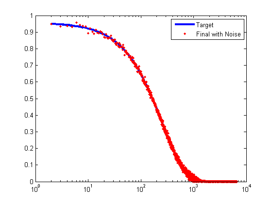
To make the CCD profile a little more realistic, we add noise according to the following formula:

$c_d \sim \mathcal{N}(\bar c_d, \min\{.001, \bar c_d/2\}).$

% Compute target CCD
ccd_stddev = min(0.01,ccd_target/2);
ccd = max(ccd_target +  randn(size(ccd_target)) .* ccd_stddev,0);

% Plot (on same axes as previous plot)
semilogx(2:maxdeg, ccd(2:end),'r.');
legend('Target','Final with Noise');

Step 4: Generate BTER model

BTER creates two edges lists, corresponding to Phase 1 and Phase 2 edges, respectively.

fprintf('Running BTER...\n');
t1=tic;
[E1,E2] = bter(nd,ccd);
toc(t1)
fprintf('Number of edges created by BTER: %d\n', size(E1,1) + size(E2,1));

Running BTER...
--- BTER HPC Set-up ---
Desired number of nodes: 100000
Desired number of edges: 1605306
Multiplier to degree-1 nodes: 1
Maximum degree: 6650
Number of groups: 137
Number of blocks: 10156
Phase 1 total weight: 3094314
Phase 2 total weight: 421610
Time for setup (sec): 0.17
Determined phase for 3515924 edges in 0.221963 seconds
Sampled 3094841 edges for phase 1 in 2.378587 seconds
Sampled 421083 edges for phase 2 in 0.642167 seconds
Removed 360 loops in 0.020099 seconds
--- BTER HPC Complete ---
Elapsed time is 3.504003 seconds.
Number of edges created by BTER: 3515564

Step 5: Create sparse matrix representation of BTER graph

Converting the edge list to an adjacency matrix is often the most expensive part in MATLAB. We separate this step because the edge list may be sufficient for many applications.

fprintf('Turning edge list into adjacency matrix (including dedup)...\n');
t2=tic;
G_bter = bter_edges2graph(E1,E2);
toc(t2);
fprintf('Number of edges in dedup''d graph: %d\n', nnz(G)/2);

Turning edge list into adjacency matrix (including dedup)...
Elapsed time is 8.560615 seconds.
Number of edges in dedup'd graph: 1090108

Step 6: Calculate metrics on BTER graph and compare to targets

% Number of nodes and edges
nnodes_bter = size(G_bter,1);
nedges = sum(nd .* (1:length(nd))');
nedges_bter = nnz(G_bter)/2;
fprintf('Comparative Results: %s versus BTER\n', graphname);
fprintf('Number of nodes: %d versus %d\n', nnodes, nnodes_bter);
fprintf('Number of edges: %d versus %d\n', nedges, nedges_bter);

% Degree disttribution
nd_bter = accumarray(nonzeros(sum(G_bter,2)),1);
maxdeg_bter = find(nd_bter>0,1,'last');
fprintf('Maximum degree: %d versus %d\n', maxdeg, maxdeg_bter);

% Clustering coefficients
[ccd_bter,gcc_bter] = ccperdeg(G_bter);
fprintf('Global clustering coefficient: %.2f versus %.2f\n', gcc_target, gcc_bter);

Comparative Results: web-NotreDame-simple versus BTER
Number of nodes: 100000 versus 100000
Number of edges: 3210611 versus 1532209
Maximum degree: 6650 versus 3177
Global clustering coefficient: 0.15 versus 0.31

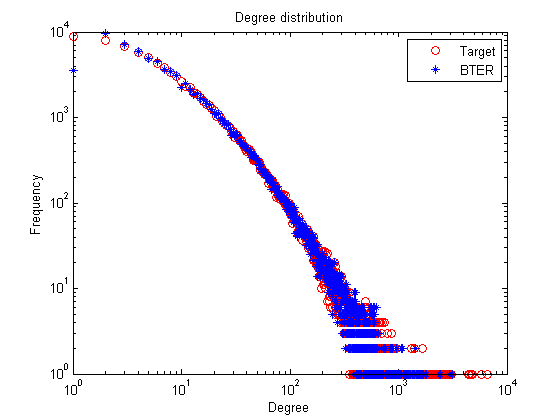
Step 7: Visualize the data

% Degree distribution
figure;
loglog(1:length(nd),nd,'ro',1:length(nd_bter),nd_bter,'b*');
title('Degree distribution');
xlabel('Degree');
ylabel('Frequency');
legend('Target', 'BTER');

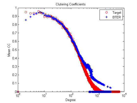
% Clustering coefficients
figure;
semilogx(1:length(ccd),ccd,'ro',1:length(ccd_bter),ccd_bter,'b*');
title('Clutering Coefficients');
xlabel('Degree');
ylabel('Mean CC');
legend('Target', 'BTER');

Note 1: Speeding up the degree distribution generation

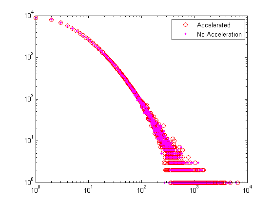
Randomized sampling for large n can be too slow. To accelerate the process, our gendegdist function assumes specified a bound such that nd(d) = round( n * pdf(d) ) for all d < bnd. Then true random sampling in the range d >= bnd is used for the remaining few nodes that need degrees assigned. If bnd is too large, however, the approximation will be highly innaccurate.

% No acceleration
tic; nd_slow = gendegdist(nnodes, pdf); toc;

% Generate a random degree distribution using the discrete PDF
bnd = 100;
tic; nd = gendegdist(nnodes,pdf,bnd); toc;

% Show the difference between accelerated and not
figure;
loglog(nd,'ro');
hold all;
loglog(nd_slow,'m.');
legend('Accelerated','No Acceleration');
xlim([1 maxdeg_bound]);

Elapsed time is 0.023331 seconds.
Elapsed time is 0.002713 seconds.

Note 2: Why we don't like power law

It's much more difficult to find power law parameters that allow both a relatively high average degree and a relatively low absolute maximum degree. Using the same parameters as above, we cannot find a $\gamma$ fot the power lab distribution such that $P(d^*) < 10^{-10}$.

gamma = degdist_param_search(avgdeg_target, maxdeg_bound, 'type', 'dpl', 'maxdeg_prbnd', tau);
fprintf('Selected gamma=%f\n', gamma);

gamma=2.000, maxdeg=10000, p(maxdeg)=6.079641e-09, avgdeg=6.0, y=678.58
gamma=2.100, maxdeg=10000, p(maxdeg)=2.551674e-09, avgdeg=4.2, y=771.04
gamma=1.900, maxdeg=10000, p(maxdeg)=1.435801e-08, avgdeg=9.0, y=536.87
gamma=1.800, maxdeg=10000, p(maxdeg)=3.353586e-08, avgdeg=14.4, y=315.81
gamma=1.600, maxdeg=10000, p(maxdeg)=1.746750e-07, avgdeg=42.8, y=123.31
gamma=1.400, maxdeg=10000, p(maxdeg)=8.255313e-07, avgdeg=137.2, y=11077.58
gamma=1.400, maxdeg=10000, p(maxdeg)=8.255313e-07, avgdeg=137.2, y=11077.58
gamma=1.700, maxdeg=10000, p(maxdeg)=7.723558e-08, avgdeg=24.4, y=64.28
gamma=1.800, maxdeg=10000, p(maxdeg)=3.353586e-08, avgdeg=14.4, y=315.81
gamma=1.650, maxdeg=10000, p(maxdeg)=1.164518e-07, avgdeg=32.2, y=6.43
gamma=1.600, maxdeg=10000, p(maxdeg)=1.746750e-07, avgdeg=42.8, y=123.31
gamma=1.675, maxdeg=10000, p(maxdeg)=9.489508e-08, avgdeg=28.0, y=22.40
gamma=1.625, maxdeg=10000, p(maxdeg)=1.427211e-07, avgdeg=37.1, y=32.44
gamma=1.662, maxdeg=10000, p(maxdeg)=1.051387e-07, avgdeg=30.0, y=10.31
gamma=1.637, maxdeg=10000, p(maxdeg)=1.289406e-07, avgdeg=34.6, y=12.94
gamma=1.656, maxdeg=10000, p(maxdeg)=1.106551e-07, avgdeg=31.1, y=7.22
gamma=1.644, maxdeg=10000, p(maxdeg)=1.225422e-07, avgdeg=33.4, y=8.24
gamma=1.653, maxdeg=10000, p(maxdeg)=1.135176e-07, avgdeg=31.6, y=6.52
gamma=1.647, maxdeg=10000, p(maxdeg)=1.194594e-07, avgdeg=32.8, y=6.99
gamma=1.652, maxdeg=10000, p(maxdeg)=1.149756e-07, avgdeg=31.9, y=6.40
gamma=1.653, maxdeg=10000, p(maxdeg)=1.135176e-07, avgdeg=31.6, y=6.52
gamma=1.651, maxdeg=10000, p(maxdeg)=1.157114e-07, avgdeg=32.1, y=6.39
gamma=1.650, maxdeg=10000, p(maxdeg)=1.164518e-07, avgdeg=32.2, y=6.43
gamma=1.651, maxdeg=10000, p(maxdeg)=1.153429e-07, avgdeg=32.0, y=6.39
gamma=1.652, maxdeg=10000, p(maxdeg)=1.149756e-07, avgdeg=31.9, y=6.40
gamma=1.651, maxdeg=10000, p(maxdeg)=1.155270e-07, avgdeg=32.0, y=6.39
gamma=1.651, maxdeg=10000, p(maxdeg)=1.151591e-07, avgdeg=32.0, y=6.39
gamma=1.651, maxdeg=10000, p(maxdeg)=1.154350e-07, avgdeg=32.0, y=6.39
Warning: Could not find ideal solution. F(X)=6.389128e+00, Exit Flag = 1.
 
Selected gamma=1.651172

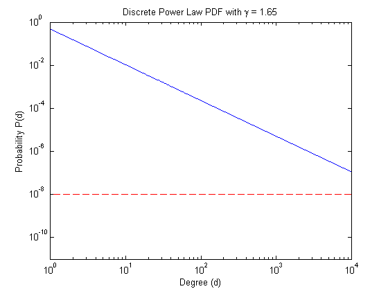
Visualizing the results shows the distance from the bound.

% Create the discrete PDF
pdf = dplpdf(maxdeg_bound,gamma);

% Visualize the PDF
figure;
loglog(pdf);
hold on;
plot([1 maxdeg_bound], [tau tau], 'r--');
tstr = sprintf('Discrete Power Law PDF with \\gamma = %.2f', gamma);
title(tstr);
xlabel('Degree (d)')
ylabel('Probability P(d)');
xlim([1 maxdeg_bound])
ylim([1e-11 1])

Now we show a few realization of the sampled degree distribution. Observe that there's very few gaps as we approach the maximum allowed degree (1e5). This results in a "cliff" in the degree distribution rather than a graduate tapering.

figure;
pos = get(gcf, 'Position');
set(gcf, 'Position', [pos(1) pos(2) 800 600]); %<- Set size
for i = 1:6
    subplot(2,3,i);
    set(gca, 'FontSize', 8);
    nd = gendegdist(nnodes,pdf);
    loglog(nd,'b.');
    xlim([1 maxdeg_bound])
    avgdeg = sum(nd .* (1:length(nd))')/sum(nd);
    maxdeg = find(nd>0,1,'last');
    tstr = sprintf('Avg Deg = %.1f, Max Deg = %d', avgdeg, maxdeg);
    title(tstr);
end

References

Published with MATLAB® R2013a

References

- BTER Implementation: T. G. Kolda, A. Pinar, T. Plantenga and C. Seshadhri. A Scalable Generative Graph Model with Community Structure, arXiv:1302.6636, March 2013, http://arxiv.org/abs/1302.6636