BTER Guide: How to create a BTER graph that matches an existing graph

By the BTER Team (Sandia National Laboratories, Livermore, CA):

April 2013

Distributed with FEASTPACK.

Sandia National Laboratories is a multi-program laboratory managed and operated by Sandia Corporation, a wholly owned subsidiary of Lockheed Martin Corporation, for the U.S. Department of Energy's National Nuclear Security Administration under contract DE-AC04-94AL85000.

Contents

Step 1: Load a graph

Some preprocessing may be needed to make the graph simple.

G = G + G'; %<- Make the graph undirected
G = spones(G); %<- Make the graph unweighted
G = spdiags(zeros(size(G,1),1),0,G); %<- Remove self-loops

We use an example graph from the SNAP collection which has already been preprocessed and is included in the distribution.

load('data/ca-AstroPh-simple');
nnodes = size(G,1);
nedges = nnz(G)/2;
fprintf('Graph name: %s\n', graphname);
fprintf('Number of nodes: %d\n', nnodes);
fprintf('Number of edges: %d\n', nedges);

Graph name: ca-AstroPh-simple
Number of nodes: 18772
Number of edges: 198050

Step 2: Compute the degree distribution

Calculate the number of nodes per degree.

nd = accumarray(nonzeros(sum(G,2)),1);
maxdegree = find(nd>0,1,'last');
fprintf('Maximum degree: %d\n', maxdegree);

Maximum degree: 504

Step 3: Calculate the clustering coefficient per degree

This can be extremely expensive, especially for large graphs. We provide C code and accompanying mex interfaces to do both exact and estimated calculations. The matlab function ccperdeg is an interface to both; see below for details. The ccperdeg function returns the clustering coefficient per degree (ccd) and the global clustering coefficient (gcc). In the second case, the value of 'nsamples' is the number of sample wedges per bin.

[ccd,gcc] = ccperdeg(G);
fprintf('Global clustering coefficient: %.2f\n', gcc);

Global clustering coefficient: 0.32

Step 4: Generate BTER model

BTER creates two edges lists, corresponding to Phase 1 and Phase 2 edges, respectively.

fprintf('Running BTER...\n');
t1=tic;
[E1,E2] = bter(nd,ccd);
toc(t1)
fprintf('Number of edges created by BTER: %d\n', size(E1,1) + size(E2,1));

Running BTER...
--- BTER HPC Set-up ---
Desired number of nodes: 18771
Desired number of edges: 198050
Multiplier to degree-1 nodes: 1
Maximum degree: 504
Number of groups: 76
Number of blocks: 2095
Phase 1 total weight: 303303
Phase 2 total weight: 52313
Time for setup (sec): 0.02
Determined phase for 355616 edges in 0.018912 seconds
Sampled 303534 edges for phase 1 in 0.185769 seconds
Sampled 52082 edges for phase 2 in 0.058720 seconds
Removed 35 loops in 0.001642 seconds
--- BTER HPC Complete ---
Elapsed time is 0.319444 seconds.
Number of edges created by BTER: 355581

Step 5: Create sparse matrix representation of BTER graph

Converting the edge list to an adjacency matrix is often the most expensive part in MATLAB. We separate this step because the edge list may be sufficient for many applications.

fprintf('Turning edge list into adjacency matrix (including dedup)...\n');
t2=tic;
G_bter = bter_edges2graph(E1,E2);
toc(t2);
fprintf('Number of edges in dedup''d graph: %d\n', nnz(G)/2);

Turning edge list into adjacency matrix (including dedup)...
Elapsed time is 0.770594 seconds.
Number of edges in dedup'd graph: 198050

Step 6: Calculate metrics on BTER graph and compare to original

% Number of nodes and edges
nnodes_bter = size(G_bter,1);
nedges_bter = nnz(G_bter)/2;
fprintf('Comparative Results: %s versus BTER\n', graphname);
fprintf('Number of nodes: %d versus %d\n', nnodes, nnodes_bter);
fprintf('Number of edges: %d versus %d\n', nedges, nedges_bter);

% Degree disttribution
nd_bter = accumarray(nonzeros(sum(G_bter,2)),1);
maxdegree_bter = find(nd_bter>0,1,'last');
fprintf('Maximum degree: %d versus %d\n', maxdegree, maxdegree_bter);

% Clustering coefficients
[ccd_bter,gcc_bter] = ccperdeg(G_bter);
fprintf('Global clustering coefficient: %.2f versus %.2f\n', gcc, gcc_bter);

Comparative Results: ca-AstroPh-simple versus BTER
Number of nodes: 18772 versus 18771
Number of edges: 198050 versus 195795
Maximum degree: 504 versus 423
Global clustering coefficient: 0.32 versus 0.33

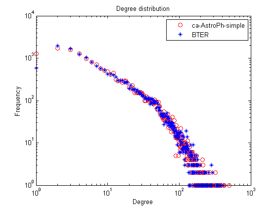
Step 7: Visualize the data

% Degree distribution
figure;
loglog(1:length(nd),nd,'ro',1:length(nd_bter),nd_bter,'b*');
title('Degree distribution');
xlabel('Degree');
ylabel('Frequency');
legend(graphname, 'BTER');

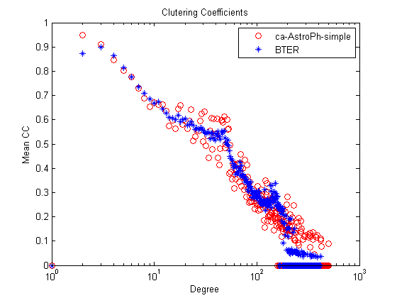
% Clustering coefficients
figure;
semilogx(1:length(ccd),ccd,'ro',1:length(ccd_bter),ccd_bter,'b*');
title('Clutering Coefficients');
xlabel('Degree');
ylabel('Mean CC');
legend(graphname, 'BTER');

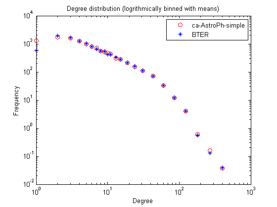
Step 7 (alternate): Visualize the results with binning

The data can be extremely crowded, especially for the higher degrees. We also include the bindata function that can be used to logrithmically bin the data. Type 'help bindata' for full instructions. We make the following parameter choices here:

binparams = {'tau', 10,'omega', 1.5, 'ybinfun', @mean, 'prebin', false};

In the binned version, the degree distibution can be non-integer and less than one because its the average value for the bin.

% Degree distribution
figure;
[xx1,yy1] = bindata([], nd, binparams{:});
[xx2,yy2] = bindata([], nd_bter, binparams{:});
loglog(xx1,yy1,'ro',xx2,yy2,'b*');
title('Degree distribution (logrithmically binned with means)');
xlabel('Degree');
ylabel('Frequency');
legend(graphname, 'BTER');

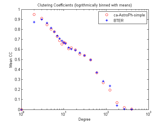
Clustering coefficients

figure;
[xx1,yy1] = bindata([], ccd, binparams{:});
[xx2,yy2] = bindata([], ccd_bter, binparams{:});
semilogx(xx1,yy1,'ro',xx2,yy2,'b*');
title('Clutering Coefficients (logrithmically binned with means)');
xlabel('Degree');
ylabel('Mean CC');
legend(graphname, 'BTER');

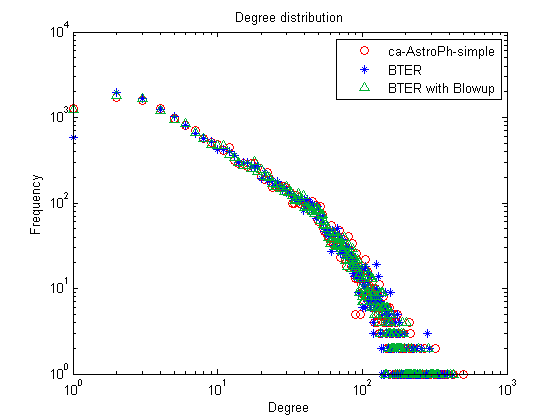
"Blowup" option in BTER for better match to degree-1 vertices

In many cases, BTER underestimates the number of degree-1 nodes. This is a well-understood problem, and we use the correction prescribed by Durak et al. (arXiv:1210.5288, 2012). We can see that now the number of degree-1 vertices is much more accurate.

[E1_alt,E2_alt] = bter(nd,ccd,'verbose',false,'blowup',10);
G_alt = bter_edges2graph(E1_alt, E2_alt);
nd_alt = accumarray(nonzeros(sum(G_alt,2)),1);
figure;
loglog(1:length(nd),nd,'ro',1:length(nd_bter),nd_bter,'b*');
hold on;
loglog(1:length(nd_alt),nd_alt,'g^','Color', [0 .7 .2]);
title('Degree distribution');
xlabel('Degree');
ylabel('Frequency');
legend(graphname, 'BTER', 'BTER with Blowup');

Larger graphs: Deduplicating the edge list

It's expensive to form a sparse adjancey matrix for very large graphs. If you want to remove duplicate edges in the edge list, we suggest the following procedure.

% Before we begin, we have to do some preprocessing to remove any loops
% from Phase 2 (cannot occur in Phase 1), and order the vertices defining
% the edges so that the least index is always first. Note that this step
% can be skipped if 'swap' and 'rmloops' options area set to true when
% running BTER.

% --- Preprocessing for Deduplication ---
% Remove loops in Phase 2
tf = (E2(:,1) == E2(:,2));
E2 = E2(~tf,:);
% Consistently order Phase 1
tf = E1(:,1) > E1(:,2);
tmp = E1(tf,2);
E1(tf,2) = E1(tf,1);
E1(tf,1) = tmp;
% Consistently order Phase 2
tf = E2(:,1) > E2(:,2);
tmp = E2(tf,2);
E2(tf,2) = E2(tf,1);
E2(tf,1) = tmp;
% --- Preprocessing Complete ---

% First, deduplicate Phase 1, which has most of the duplication
E1_dedup = unique(E1,'rows');
fprintf('Number of duplicates in Phase 1: %d\n', size(E1,1) - size(E1_dedup,1));

% Next, deduplicate Phase 2, which does not have much duplication
E2_dedup = unique(E2,'rows');
fprintf('Number of duplicates in Phase 2: %d\n', size(E2,1) - size(E2_dedup,1));

% Finally, remove any duplicates between the 2 phases.
E_dedup = unique([E1_dedup; E2_dedup], 'rows');
fprintf('Number of duplicates across Phasees: %d\n', ...
    size(E1_dedup,1) + size(E2_dedup,1) - size(E_dedup,1));
fprintf('Final number of edges: %d\n', size(E_dedup,1));

Number of duplicates in Phase 1: 157937
Number of duplicates in Phase 2: 776
Number of duplicates across Phasees: 1073
Final number of edges: 195795

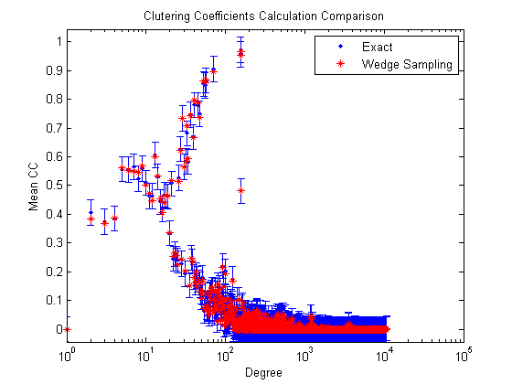
Larger graphs: Calculating the clustering coefficients

For larger graphs, calculating the clustering coefficient exactly can be extremely expensive. Here we compare the exact and estimated clustering coefficients using the two different methods.

% Load a bigger graph
load('data/web-NotreDame-simple');
nnodes = size(G,1);
nedges = nnz(G)/2;
fprintf('Graph name: %s\n', graphname);
fprintf('Number of nodes: %d\n', nnodes);
fprintf('Number of edges: %d\n', nedges);

% Calculate the clustering coefficients _exactly_.
tic;
[ccd0,gcc0] = ccperdeg(G,'nsamples',0);
t = toc;
fprintf('      Exact GCC: %e (%f seconds to compute) \n', gcc0, t);

% Calculate the clustering coefficients using wedge sampling.
nsamples = 2000;
tic;
[ccd,gcc] = ccperdeg(G,'nsamples',nsamples);
t = toc;
fprintf('  Estimated GCC: %e (%f seconds to compute) \n', gcc, t);

% Compute the bound on the error and check results.
delta = 0.001; %<-Corresponding to 99.9% confidence.
errorbound = sqrt(log(2/delta)/(2*nsamples));
fprintf(' Expected error: %e (with 99.9%% confidence)\n', errorbound);
fprintf('  Max CCD error: %e\n', max(abs(ccd-ccd0)));
fprintf('      GCC error: %e\n', abs(gcc-gcc0));

% Visualize the differences
figure;
e = ones(size(ccd0));
errorbar(1:length(ccd0),ccd0,errorbound*e,errorbound*e,'b.');
set(gca,'XScale','log')
hold on;
plot(1:length(ccd),ccd,'r*');
xl = xlim;
xlim([1 xl(2)]);
ylim([-errorbound 1+errorbound]);
title('Clutering Coefficients Calculation Comparison');
xlabel('Degree');
ylabel('Mean CC');
legend('Exact', 'Wedge Sampling');

Graph name: web-NotreDame-simple
Number of nodes: 325729
Number of edges: 1090108
      Exact GCC: 8.767355e-02 (2.091621 seconds to compute) 
  Estimated GCC: 8.747799e-02 (0.535013 seconds to compute) 
 Expected error: 4.359158e-02 (with 99.9% confidence)
  Max CCD error: 2.666742e-02
      GCC error: 1.955560e-04

References

Published with MATLAB® R2013a