Thanks to Rasmus Bro, Nikos Sidiropoulos, Aravindan Vijayaraghavan, and Aditya Bhaskara for helpful discussions on this topic and contributions to this post.
Summary
In many papers on tensor decomposition since 2014, the simultaneous diagonalization algorithm is incorrectly referenced as Jennrich’s algorithm. This method should not be attributed to Jennrich or even Harshman (1970) but instead referred to simply as the simultaneous diagonalization method. The best single reference for the algorithm is Leurgans, Ross, and Abel (1993), though other relevant papers can also be cited as discussed further in this post.
Background
The CP tensor decomposition was first discovered by Hitchcock (1927) and then rediscovered independently in 1970 by two groups who also each proposed the same algorithm for computing it:
R. A. Harshman (1970). Foundations of the PARAFAC procedure: Models and conditions for an “explanatory” multi-modal factor analysis, UCLA working papers in phonetics, 16:1-84
J. D. Carroll, and J. J. Chang (1970).Analysis of individual differences in multidimensional scaling via an N-way generalization of “Eckart-Young” decomposition, Psychometrika, 35:283-319
Harshman’s paper credits Robert Jennrich for the algorithm (and a proof of uniqueness).
The algorithm that Jennrich proposed in Harshman (1970) is not Simultaneous Diagonalization but instead Alternating Least Squares,
the same as that proposed by Carroll and Chang.
Here is an excerpt from Harshman (1970) that specifies the algorithm: 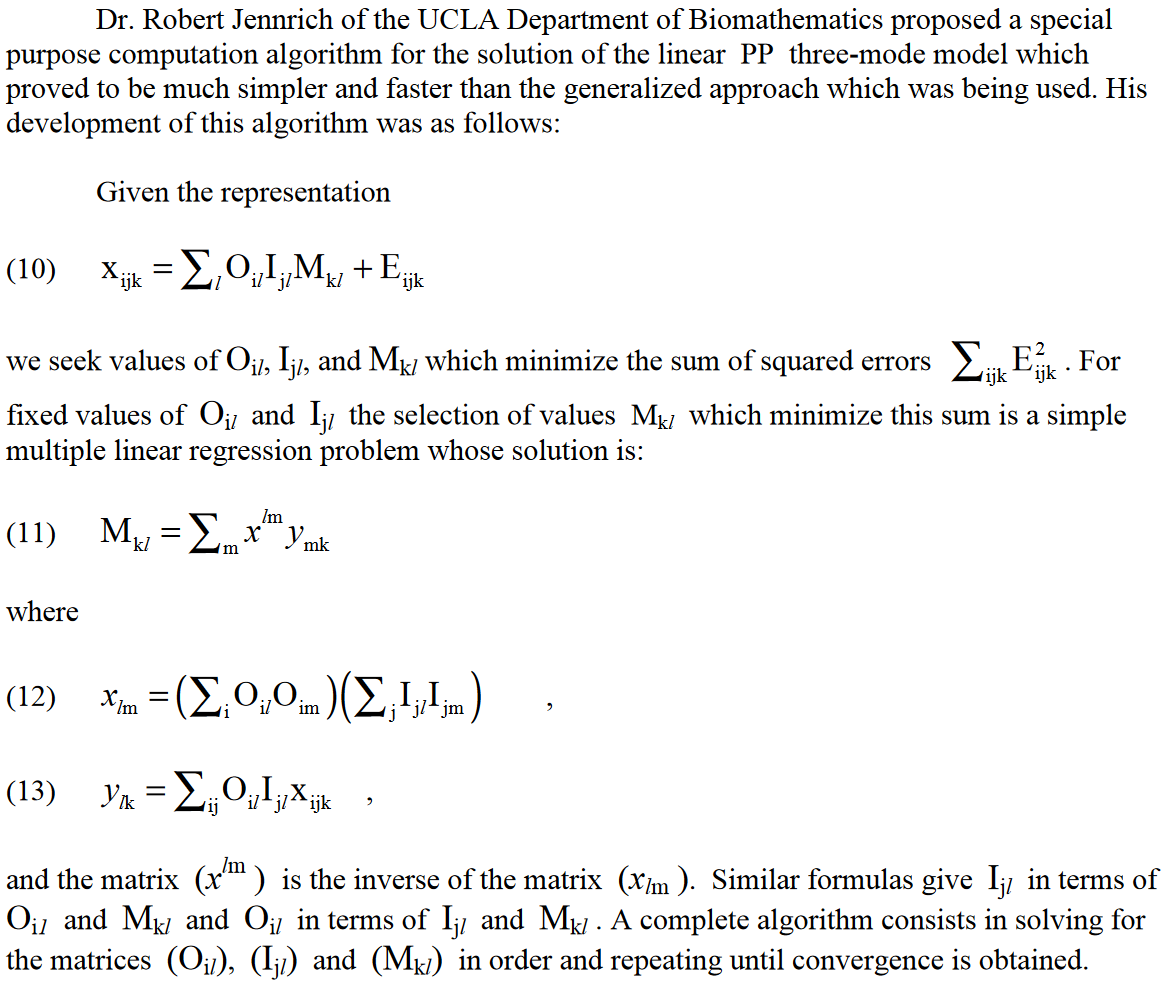
The simultaneous diagonalization algorithm wrongly credited to Jennrich has an interesting history that is discussed in detail in Appendix 6.A of A. Smilde, R. Bro, and P. Geladi (2004), Multi-Way Analysis: Applications in the Chemical Sciences, Wiley. See also the background discussion in L. De Lathauwer, B. De Moor, and J. Vandewalle (2004), Computation of the Canonical Decomposition by Means of a Simultaneous Generalized Schur Decomposition, SIAM J. Matrix Analysis and Applications, 26:295-327. (see also Further Reading below).
For these reasons, this method has no obvious progenitor for whom it should be named, and the most apropos single reference is
- S. E. Leurgans, R. T. Ross, and R. B. Abel (1993). A Decomposition for Three-Way Arrays, SIAM J. Matrix Analysis and Applications, 14:1064-1083
The “real” Jennrich’s algorithm is BETTER!
The simultaneous diagonalization only works for three-way tensors and
is numerically finicky.
There are robust MATLAB implementations of simultaneous diagonalization in both N-way Toolbox (nwy_dtld) and TensorLab (tlb_sd), so we
compare these to the “real” Jennrich’s algorithm,
which is the well-known Alternating Least Squares (ALS).
We do this on a tensor of size $25 \times 20 \times 15$
with rank $r=10$ and 20% noise and correlated columns
in the factor matrices (congruency of 0.8).
The ALS method achieves a better fit of 0.81 versus 0.80
for simultaneous diagonalization and, more importantly,
a much better correlation with the noise-free solution of 0.925 versus 0.651.
(Full details are given at the end of this posting.)
A Connection with respect to Uniqueness
One point of similarity between the paper of Leurgans-Ross-Abel and Jennrich (via Harshman) is that they proved uniqueness of the CP tensor decomposition under similar circumstances.
Jennrich (Harshman 1970): The rank-$R$ decomposition $X = [[A,B,C]]$ is unique (up to permutation and scaling) if $\text{rank}(A) = \text{rank}(B) = \text{rank}( C ) = R$.
Leurgans-Ross-Abel (1993): The rank-$R$ decomposition $X = [[A,B,C]]$ is unique (up to permutation and scaling) if $\text{rank}(A) = \text{rank}(B) = $ and $\text{K-rank}( C ) = 2$ (i.e., any pair of columns in $C$ are linearly independent).
There are two important differences between these results.
(1) There is no connection between Jennrich’s result and the algorithm he proposed. In contrast, the simultaneous diagonalization algorithm of Leurgans-Ross-Abel was directly connected to their theory.
(2) The condition on $C$ is stricter in Harshman’s version.
A Stepping Stone
There is another paper by Harshman that derives the same result as Leurgans-Ross-Abel:
- R. A. Harshman. Determination and Proof of Minimum Uniqueness Conditions for PARAFAC1, UCLA working papers in phonetics, Vol. 22, pp. 111-117, 1972.
It does credit Robert Jennrich and David Cantor for constructive feedback, but the credit for this result goes to Harshman himself. So we add another uniqueness milestone:
- Harshman (1972): The rank-$R$ decomposition $X = [[A,B,C]]$ is unique (up to permutation and scaling) if $\text{rank}(A) = \text{rank}(B) = $ and $\text{K-rank}( C ) = 2$ (i.e., any pair of columns in $C$ are linearly independent).
A few comments are in order.
(1) No algorithm is provided, though the proof is constructive.
(2) Leurgans-Ross-Abel (1993) did not cite Harshman (1972), and their proof seems to have been developed independently.
An Aside on Uniqueness
As an aside, we should also note a more general result which does not come with an algorithm for its computation. The reference is
- J. B. Kruskal (1977). Three-way arrays: rank and uniqueness of trilinear decompositions, with application to arithmetic complexity and statistics, Linear Algebra and its Applications, 18:95-138
The result is
- Kruskal (1977): The rank-$R$ decomposition $X = [[A,B,C]]$ is unique (up to permutation and scaling) if $\text{K-rank}(A) + \text{K-rank}(B) + \text{K-rank}( C ) \geq 2R+2$ where K-rank is defined to be the minimum value $K$ such that any $K$ columns are linearly independent.
Further Reading
A nice explanation of the uniqueness conditions and algebraic solution is given here:
- J. M. F. ten Berge, and J. N. Tendeiro (2009), The link between sufficient conditions by Harshman and by Kruskal for uniqueness in Candecomp/Parafac, J. Chemometrics, 23:321-323
Other papers that are often credited in the evolution of these ideas are:
E. Sanchez and B. Kowalski (1990), Tensorial resolution: A direct trilinear decomposition, J. Chemometrics, 4:29-45
R. Sands and F. Young (1980), Component models for three-way data: An alternating least squares algorithm with optimal scaling features, Psychometrika, 45:39-67.
Perhaps the most general version of the algebraic solution method is provided here:
- I. Domanov, and L. Lathauwer (2014), Canonical Polyadic Decomposition of Third-Order Tensors: Reduction to Generalized Eigenvalue Decomposition, SIAM J. Matrix Analysis and Applications, 35:636-660
Details on Experimental Results
Setup
We create a three-way approximately low-rank tensor with the following characteristics. Size is 25 x 20 x 15. X = 80% Xtrue + 20% Normal-Distributed Noise. Xtrue = rank-10 tensor with factors [[A,B,C]] with normalized columns and such that the dot products between any two columns of A (or B or C) is exactly 0.8. (For this we use the method described by Tomasi and Bro (2006) and implemented in the Tensor Toolbox as
matrandcong.)We compare the ALS method
tlb_alsfrom TensorLab, with two simultaneous diagonalization (SD) methods:tlb_sdfrom TensorLab andnwy_dtldfrom N-way ToolboxThe correlation score of the computed solution and the true solution is computed via the
scorefunction in Tensor Toolbox. A score of 1.0 is ideal, and a score of zero indicates no correlation.We run each method 10 times and report the best fit and correlation score of the 10 runs. Note that
nwy_dtlddoes not have an option to set the initial guess.
Output
TIME
| Method | tlb_als | tlb_sd | nwy_dtld |
|---|---|---|---|
| Run 1 | 0.046 | 0.036 | 0.060 |
| Run 2 | 0.018 | 0.023 | 0.019 |
| Run 3 | 0.024 | 0.010 | 0.016 |
| Run 4 | 0.017 | 0.008 | 0.017 |
| Run 5 | 0.016 | 0.021 | 0.016 |
| Run 6 | 0.012 | 0.010 | 0.016 |
| Run 7 | 0.021 | 0.009 | 0.017 |
| Run 8 | 0.023 | 0.015 | 0.016 |
| Run 9 | 0.016 | 0.011 | 0.015 |
| Run 10 | 0.019 | 0.010 | 0.016 |
| SUM | 0.212 | 0.153 | 0.206 |
FIT
| Method | tlb_als | tlb_sd | nwy_dtld |
|---|---|---|---|
| Run 1 | 0.811 | 0.800 | 0.793 |
| Run 2 | 0.811 | 0.800 | 0.793 |
| Run 3 | 0.808 | 0.797 | 0.793 |
| Run 4 | 0.811 | 0.796 | 0.793 |
| Run 5 | 0.812 | 0.800 | 0.793 |
| Run 6 | 0.811 | 0.797 | 0.793 |
| Run 7 | 0.811 | 0.796 | 0.793 |
| Run 8 | 0.812 | 0.800 | 0.793 |
| Run 9 | 0.812 | 0.799 | 0.793 |
| Run 10 | 0.812 | 0.800 | 0.793 |
| MAX | 0.812 | 0.800 | 0.793 |
SCORE
| Method | tlb_als | tlb_sd | nwy_dtld |
|---|---|---|---|
| Run 1 | 0.910 | 0.643 | 0.568 |
| Run 2 | 0.850 | 0.646 | 0.568 |
| Run 3 | 0.740 | 0.544 | 0.568 |
| Run 4 | 0.871 | 0.520 | 0.568 |
| Run 5 | 0.921 | 0.638 | 0.568 |
| Run 6 | 0.876 | 0.608 | 0.568 |
| Run 7 | 0.896 | 0.605 | 0.568 |
| Run 8 | 0.875 | 0.651 | 0.568 |
| Run 9 | 0.846 | 0.566 | 0.567 |
| Run 10 | 0.925 | 0.642 | 0.568 |
| MAX | 0.925 | 0.651 | 0.568 |
Source Code
%% Comparing ALS and SD

%% Setup path
% Be sure to add the Tensor Toolbox (Version 3.2.1), the N-Way Toolbox, and
% TensorLab (Version 3.0) to your path in that order. In the search path,
% tensorlab should be above, nway331, which is above tensor_toolbox.

%% Create a test problem
m = 25; n = 20; p = 15; r = 10;

rng('default') %<- For reproducibility, feel free to omit

info = create_problem('Size',[m n p],'Num_Factors',r,'Noise',0.2,...
    'Factor_Generator', @(m,n) matrandcong(m,n,0.8), ...
    'Lambda_Generator', @ones);

X = info.Data;
Mtrue = arrange(info.Soln);

%% Run experiments

rng('default') %<- For reproducibility, feel free to omit

ntrials = 10;
results = cell(ntrials,1);
for i = 1:ntrials

    U1 = randn(m,r);
    U2 = randn(n,r);
    U3 = randn(p,r);
    Minit = {U1,U2,U3};

    tic
    M = cpd_als(X.data,Minit);
    results{i}.tlb_als.time = toc;
    M = ktensor(M);
    results{i}.tlb_als.fit = 1 - norm(X-full(M))/norm(X);
    results{i}.tlb_als.score = score(M,Mtrue,'lambda_penalty',false);

    tic
    M = cpd3_sd(X.data,Minit);
    results{i}.tlb_sd.time = toc;
    M = ktensor(M);
    results{i}.tlb_sd.fit = 1 - norm(X-full(M))/norm(X);
    results{i}.tlb_sd.score = score(M,Mtrue,'lambda_penalty',false);

    % No way to set the initial guess for DTLD
    tic
    [A,B,C] = dtld(X.data,r);
    results{i}.nwy_dtld.time = toc;
    M = ktensor({A,B,C});
    results{i}.nwy_dtld.fit = 1 - norm(X-full(M))/norm(X);
    results{i}.nwy_dtld.score = score(M,Mtrue,'lambda_penalty',false);

end

%% Print out results in a way compatible with markdown

method = fieldnames(results{1});
measure = fieldnames(results{1}.(method{1}));
summary = {'sum','max','max'};

for i = 1:length(measure)

    fprintf('\n');
    fprintf('### %s \n\n', upper(measure{i}));

    fprintf('| Method |');
    for j = 1:length(method)
        fprintf(' %8s |', method{j});
    end
    fprintf('\n');

    fprintf('| ------ |');
    for j = 1:length(method)
        fprintf(' -------- |');
    end
    fprintf('\n');

    for k = 1:size(results,1)
        fprintf('| Run %2d |',k);
        for j = 1:length(method)
            fprintf(' %8.3f |', results{k}.(method{j}).(measure{i}));
        end
        fprintf('\n');
    end

    fprintf('| %4s   |',upper(summary{i}));
    for j = 1:length(method)
        fprintf(' %8.3f |', feval(summary{i},(cellfun(@(x) x.(method{j}).(measure{i}), results))));
    end

    fprintf('\n');

end

fprintf('\n');